Joints
This section contains joints that can be used to create, for example, linear motions similar to cylinders, rotary movements, wheel connections, etc.
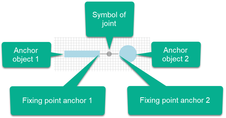
Joints always define the relationship between two physics objects. These two objects are the anchor objects of the joint.
Drawing joints
Some joints have a master object and a slave object. When you draw a joint, some settings are transferred from the master object to the slave object. The start object, where you start drawing the joint, is always the master object as well.
To attach a joint to two objects, proceed as follows:
- Select a joint
- Move the mouse to the first anchor point for the joint in the master object, press and hold the left mouse button.
- Move the mouse to the second anchor point in the slave object and release the mouse button.
The following example shows a prismatic joint.
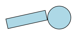
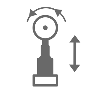
Prismatic joint
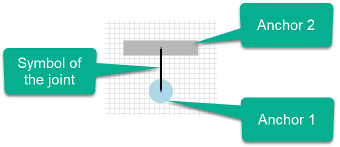
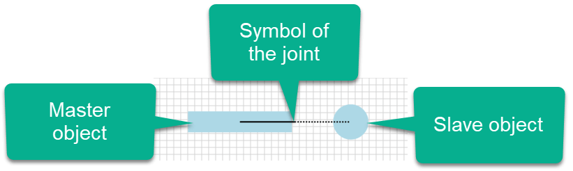
The prismatic joint is used for cylinders, for example. Below you can see the symbol of the joint:
Examples of this type of joint are:
- Cylinders
- Elevators
- Lifting platforms
- Sliding doors
- Feeds for drilling rigs
- Linear movements of grippers
- Implementation of a weigh scale
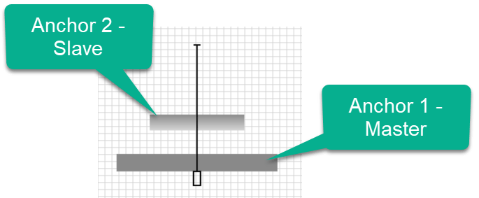
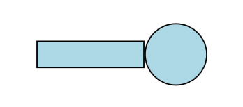
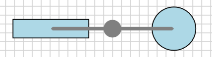
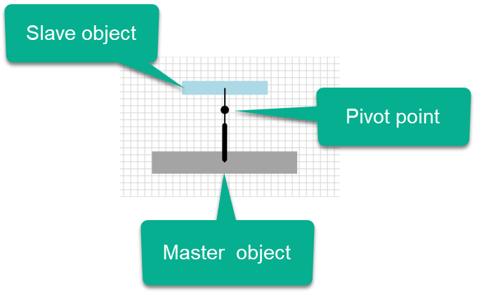
The following image shows two objects which are connected by a "prismatic joint". The left object is the master object. From this object, the second object is moved along the line of the joint symbol.
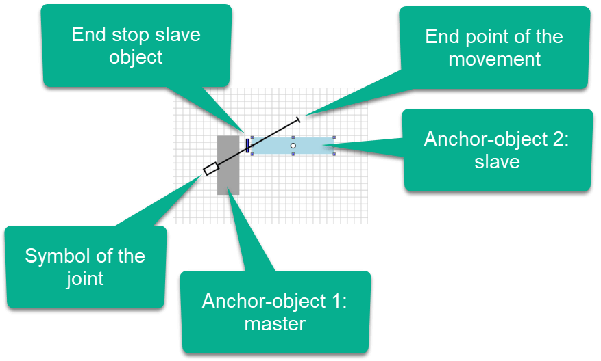
When you select the second anchor object (slave), an additional symbol appears which symbolizes the stop. When you rotate the object, the stop also rotates, so it always remains on the same side of the object. Depending on how a movement looks like, it may be necessary to rotate the slave object in order to have the stop at the correct position.
Changing the length of the "prismatic joint:
There are three ways to adjust the length of the movement.
First option
The first option is to select and move the slave object. When you move the object beyond the current end of the movement, the length of the movement is adjusted.
However, you cannot use this method to shorten the length.
Second option
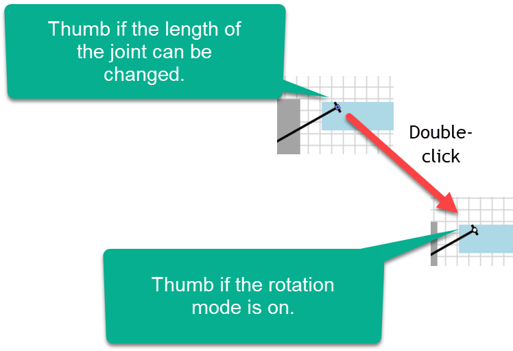
With the second option, you select the symbol of the joint and then move the mouse to the end. Now click on the thumb and hold down the left mouse button. The appearance of the joint symbol changes and the current length is displayed in pixels. Now you can use the mouse to lengthen or shorten the travel distance. Shortening is only possible as long as the stop side of the slave object is still within the travel path.
Third option
It is also possible to change the length in the properties.
To do this, select the joint and then change the "Length linear movement" property.
Changing the gradient or angle of the "prismatic joint":
There are three ways to adjust the gradient of the movement.
First option The first option is to select and move the slave object. The linear movement is also moved with the slave object. The same applies if the position of the master object is changed.
Second option With the second option, you double-click the symbol of the joint or the selected symbol. The selection thumbs indicate that the rotation mode is active.
In this mode you can now change the gradient. The position of the slave object is adjusted.
Third option The third option is to change the gradient in the properties.
To do this, select the joint and then change the "Rotation" property.
Using the motor of the "prismatic joint":
The linear joint has a motor that can be set using the "Motor" property in the property section "Physics properties -> General -> Motor settings".
The motor speed (in m/s) can be specified via an operand; the value is read from the operand. In this way, it is also possible to specify a constant if the speed does not have to be variable.
With the property "Speed divisor" you can adapt the speed specification for the simulation by means of an operand without having to change the value of the operand. The speed specified in the operand is divided by the value in "Speed divisor". This may be necessary, for example, if the motion is too fast in reality and therefore cannot be recreated in the simulation.
The movement of the slave object is controlled by operands. Because the value is read from the operand, the constant '1' can also be specified for a permanent movement.
Limit switches and sensors of the "prismatic joint": The joint has numerous sensors. This allows the end positions to be evaluated, the position of the slave object as an analog value and much more.
With the sensor for the position, it can be useful to specify a scaling range in order to generate values similar to those in the real system. It does not matter whether the length of the movement corresponds to the length of the real system.
Example A linear movement with a length of 4m is present in a system. The position sensor provides values from 0 to 4000. We want to simulate this in the virtual PLC-Lab system.
The following specification is made in the property "Sensor position in pixels":
0-4000 IM.MW2
As a result, the position of the slave object is scaled to the range 0-4000 and then written to the word operand MW2.
Because of the scaling, the length of the linear movement within the simulation is irrelevant. You get the same sensor data as you would in the real system.
Meaning of the property "Anchor objects collide".
As the name of the property suggests, you can make the master object and the slave object collide by activating this property. The property was selected in the following image:
Now the same arrangement, but the two objects do not collide because the property is not selected:

Here the slave object is not stopped by the master object.
If the two anchor objects collide and still the zero point of the linear movement has to be reached, you can often achieve this by rotating the master object. You can see this in the following image. The master object is rotated by 180° so that the starting point of the movement is in the direction of the position of the slave object.
Rotating master object and slave object
In many cases, an arrangement consisting of two objects linked by a linear motion link needs to be mirror-inverted. An example is the left and right part of a sliding door.
In such cases, the two linked objects are combined into a drawing group, copied, and then rotated.
This can be seen in the following video:
Stringing together linear movements Gripper arrangements often consist of a horizontal and vertical movement. In such a case, the slave object of the horizontal movement is also the master object of the vertical movement of the gripper.
Below is a video showing the structure of such a gripper arrangement:
If the gripper is not implemented with a magnet, but with gripper arms, then additional connections are attached to the slave object of the vertical movement, e.g. for rotary movements. In this case it is important that the mass of the slave object is increased by increasing its density. Otherwise the structure becomes unstable.
The following video shows the structure of a gripper with a gripper pliers. Note the explicit density setting at 7:14 min. into the video:
Tips for placing the slave object
The slave object is the dynamic part of the linear movement. The drawing position of this object is also the starting position at the start of the simulation.
If you want to change the drawing position of the slave object, the best way to do this is to use the arrow keys on the keyboard. To do this, select the object and use the arrow keys to change its position. When you have reached the starting position of the linear movement and then move beyond it, the direction of the linear movement changes. You should then simply go back one position (i.e. press the arrow key in the opposite direction); you will then have reached the zero point of the linear movement. You can see this below:
The arrow keys can only move an object vertically or horizontally. If the linear movement has a certain gradient, then it is very difficult to move the slave object without changing the gradient of the movement.
In such a case, the slave object should be provided with a stencil, which ensures that a displacement is only possible in the set angle of the linear movement.
The following steps are necessary to provide objects with such a stencil:
- Select all objects that you want to assign to the stencil. To select several objects, press and hold the Shift key. Then click on the individual objects with the mouse. Now select the symbol of the joint.
- Now you can release the Shift key. Within the list of actions, select the action "Set stencil".
- In the PLC-Lab status field a message appears that the stencil has been set.
- Now the objects can only be changed in position alongside a line. This is also true for changes with the mouse and with the arrow keys on the keyboard.
If you want to position the objects freely again, select them and select the action "Reset stencil".
The following video shows how to set and reset a stencil:
Implementing a weigh scale with a prismatic joint
The prismatic joint has the sensor "force in Newton". You can specify an operand for this sensor. In these operands the current value of the force in Newton is written, which the connection needs to hold the current position or to execute a potential movement.
If, for example, the linear connection is arranged vertically and the slave anchor does not move, then the value of the force required to hold this position is written into the sensor.
Below is a prismatic joint arranged vertically:
The second anchor object is located approximately in the center of the joint. The sensor "Force in N" was assigned a word operand. This word operand is also specified at a tacho object. The linear connection does not execute any movement, i.e. the constant 0 is specified at the two properties "Operand movement to minimum" and "Operand movement to maximum".
At the start of the simulation you can see the following image:

The tacho object indicates that a force of 2 Newtons is required to hold anchor 2 in position.
The next step is to place rectangles of identical size with different densities (and thus different masses) on the second anchor object.
By placing the rectangles on the second anchor, the linear connection requires a higher force to hold the position. This force is displayed in the tacho object. Depending on the mass of the object, this force is different and thus a measure of its weight.
Info
If the slave object moves and meets the limit of the linear connection, the force increases until the maximum force of the linear connection is reached.
Automatic positioning with a prismatic joint (V1.5.4.0 or higher)
With the help of automatic positioning, a prismatic joint can be set to a specific position. This is similar to a stepper motor control. Furthermore, positioning relative to the current position is also possible. The properties required for this functionality can be found in the "Positioning" section.
Meaning of the properties within the "Positioning" section
Enable Positioning
A Boolean operand or a constant can be specified at this property. As soon as the operand has the value '1' (true), the positioning is active. The same applies if the constant '1' is specified. If the positioning is active, the linear movement can no longer be controlled via the two operands "Movement to minimum" or "Movement to maximum". In addition, some properties such as "Impulse behaviour" and "Reverse velocity if status of operands is zero" are deactivated. If the operand changes from '1' to '0' during positioning, the positioning is stopped.
Adopt positioning data
A Boolean operand must be specified for this property. With a pos. edge of the operand and activated positioning, the positioning process is started.
Position specification
Operand for the specification of the position increments. The value is read from the specified operand. The specification of a constant > 0 is not allowed. Depending on the positioning mode, the value is used as absolute position or relative position change. The specification of a range is not possible! A range at the position sensor of the connection for linear movement is used.
Position mode
Operand or constant for specifying the positioning mode to be used.
| Mode | Meaning |
|---|---|
| 0 | No function |
| 1 | Positioning via absolute value. The value at the position specification is interpreted as absolute position value. |
| 2 | Positioning via relative value. The value at the position specification is interpreted as a relative position value. The direction is determined via the property "Direction for positioning". |
Direction for positioning
Operand to specify the direction of movement for relative positioning.
| Value | Meaning |
|---|---|
| 0 | Movement to the maximum. |
| 1 | Movement ro the minimum. |
Sensor Positioning done
Operand becomes true as soon as a positioning job is completed. This means that the position specified by the position specification (absolute or relative) has been reached. The operand remains true until new position data is set, the position is changed or the positioning is deactivated.
Set the maximum speed for positioning
Within the section "Motor Settings" a constant or an operand can be specified at the property "Speed in m/s". This property is also evaluated during automatic positioning.
If the value of the operand or constant is identical to 0, then positioning is performed at maximum speed. If a value > 0 is present, then the maximum speed is limited to this value during positioning.
Example for absolute positioning
In the following example a lifting platform is to be positioned absolutely. The lifting platform can be adjusted to any height between 0 and 250 cm.
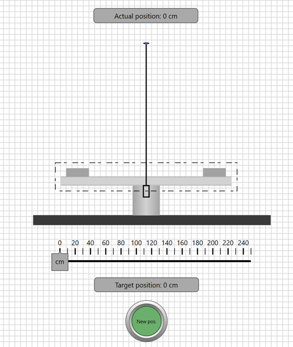
The platform of the lift is moved vertically by means of a prismatic joint. The length of the joint is set to 250, so no scaling range is necessary at the "Sensor position in pixels" property. If a scaling range would be necessary, then the range specified at this sensor would also be used for the position data of the positioning.
The following operands are used in the example:
| Symbol | Operand | Meaning |
|---|---|---|
| GoToNewPos | E0.0 | A pos. edge of this operand starts the positioning. |
| NewPosReached | E0.1 | If the positioning is done, this operand has the status '1'. |
| ActualPos | EW2 | This word operand contains the current position of the lift, in the range 0 to 250. |
| TargetPos | EW4 | The absolute target position to be approached by the lift, in the range 0 to 250. |
Since the example is to run without PLC program or GRAFCET, inputs of the Sim-Device are used.
The example is installed with PLC-Lab. See also: Positioning absolute
Settings within the motor of the prismatic joint
Below are the settings of the motor properties of the prismatic joint.
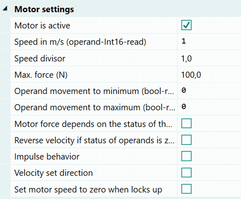
The speed is limited to 1 m/s, thus a smooth positioning is achieved. The properties for the movement to the minimum and to the maximum are each assigned the constant '0', because these are not used. If the lifting platform is to be moved manually, then the corresponding operands must be entered here. However, these would only be considered if the positioning is not active.
Settings within the sensors of the prismatic joint
Only the sensor "position in pixels" is necessary. Here the operand with the symbol "ActualPos" must be specified.
Settings within the "Positioning" section
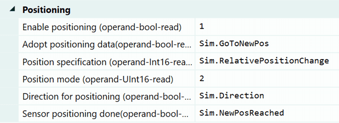
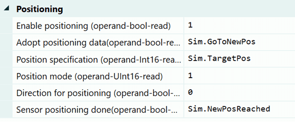
Now to the settings within the "Positioning" section. These are shown below:
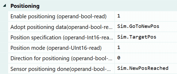
The constant '1' is specified at the property "Enable positioning", because in the example the lifting platform is to be changed in position exclusively by specifying a position value. A manual change is not intended. If this were desired, then a bit operand could be specified at the property and thus switch between manual movement and automatic positioning. In the same way, the positioning could be stopped immediately with the help of the operand. This is also omitted in this example for the sake of simplicity.
The position data should be taken over at a positive edge at the operand "GoToNewPos" and the positioning should be started. Thus, this must be specified at the property "Adopt positioning data".
Since only absolute positioning is used in the example, the constant '1' can be specified in the "Positioning mode" property.
Finally, the operand "NewPosReached" must be entered at "Sensor positioning done". This operand is set to true as soon as the positioning is completed. The operand is filled in into the illuminated switch and thus signals that the position has been reached.
Simulation of the example
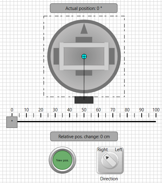
All settings are now complete and the system can be simulated. This can be seen below.
The position to be approached in each case is set with the aid of the slider and the positioning is started via the button. As soon as the position is reached, this is signalled by the illuminated switch.
Relative positioning example
In the following example, a lifting platform is to be positioned relative to the current position. The offset to the current position can be adjusted from 1 to 50 cm. A rotary switch is used to select whether the movement should be towards the maximum (up) or the minimum (down).
The platform of the lift is moved vertically by means of a prismatic joint. The length of the joint is set to 250, so no scaling range is necessary at the "Sensor position in pixels" property. If a scaling range would be necessary, then the range specified at this sensor would also be used for the position data of the positioning.
The following operands are used in the example:
| Symbol | Operand | Meaning |
|---|---|---|
| GoToNewPos | E0.0 | A pos. edge of this operand starts the positioning. |
| NewPosReached | E0.1 | If the positioning is done, this operand has the status '1'. |
| Direction | E0.2 | 0: Movement to the maximum, 1: Movement to the minimum. |
| ActualPos | EW2 | This word operand contains the current position of the lift, in the range 0 to 250. |
| TargetPos | EW4 | The target position relative to the current position, in the range 0 to 50. |
Since the example is to run without PLC program or GRAFCET, inputs of the Sim-Device are used.
The example is installed with PLC-Lab. See also: Positioning relative
Settings within the motor of the prismatic joint
Below are the settings of the motor properties of the prismatic joint.
The speed is limited to 1 m/s, thus a smooth positioning is achieved. The properties for the movement to the minimum and to the maximum are each assigned the constant '0', because these are not used. If the lifting platform is to be moved manually, then the corresponding operands must be entered here. However, these would only be considered if the positioning is not active.
Settings within the sensors of the prismatic joint
Only the sensor "position in pixels" is necessary. Here the operand with the symbol "ActualPos" must be specified.
Settings within the "Positioning" section
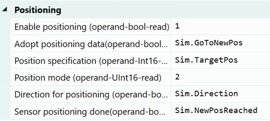
Now to the settings within the "Positioning" section. These are shown below:
The constant '1' is specified at the property "Enable positioning", because in the example the lifting platform is to be changed in position exclusively by specifying a relative position value. A manual change is not intended. If this were desired, then a bit operand could be specified at the property and thus switch between manual movement and automatic positioning. In the same way, the positioning could be stopped immediately with the help of the operand. This is also omitted in this example for the sake of simplicity.
The position data should be taken over at a positive edge at the operand "GoToNewPos" and the positioning should be started. Thus, this must be specified at the property "Adopt positioning data".
Since only relative positioning is used in the example, the constant '2' can be specified in the "Positioning mode" property.
The operand "Direction" is specified at the property "Direction for positioning". If this has the status '0', then the relative position change is executed towards the maximum (i.e. upwards). If the operand has the status '1', then the movement is towards the minimum and therefore downwards.
Finally, the operand "NewPosReached" must be entered at "Sensor positioning done". This operand is set to true as soon as the positioning is completed. The operand is filled in into the illuminated switch and thus signals that the position has been reached.
Simulation of the example
All settings are now complete and the system can be simulated. This can be seen below.
The offset to be approached in each case is set with the aid of the slider and the positioning is started via the button. As soon as the position is reached, this is signalled by the illuminated switch.
Revolute joints
A revolute joint is used, among other things, to implement the following system components:
- Revolute joints
- Fan with variable speed
- Rotary movement with position sensor
- Tilting devices
- Revolving doors
- Variable ramps
- Barriers
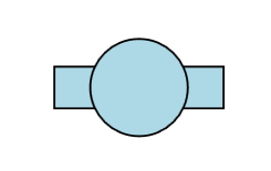
You can freely adjust the pivot point of the joint. Below you can see the principle symbol of the joint:

The following image shows two objects which are connected by a "revolute joint". The lower object is the master object, which in most cases will be a fixed object. A solid line leads from the master object to the pivot point. This is symbolized by a colored circle with a cross. The connecting lines to the slave object are dotted. The slave object is the object that rotates around the pivot point.

Changing the position of the pivot point of the "revolute joint"
You can freely position the pivot point of the joint. To do this, select the circle symbolizing the pivot point and move it with the mouse.
In the following example, the pivot point is placed in the center of the slave object.

Now an example where the pivot point is placed outside the slave object.

The examples show that very different rotary movements can be implemented by freely positioning the pivot point.
Using the motor of the revolute joint
The joint has a motor that can be set using the "Motor" property in the property section "Physics properties -> General -> Motor settings". The motor speed (in rpm) can be specified via an operand; the value is read from the operand. In this way, it is also possible to specify a constant if the speed does not have to be variable.
With the property "Speed divisor" you can adapt the speed specification for the simulation by means of an operand without having to change the value of the operand. The speed specified in the operand is divided by the value in "Speed divisor". This may be necessary, for example, if the motion is too fast in reality and therefore cannot be recreated in the simulation.
The right/left rotation of the slave object is controlled via operands. Because the value is read from the operand, the constant '1' can also be specified for a permanent rotation. Please note, however, that only one direction of rotation may be active at any one time. If both directions of rotation are active, there is no rotary movement.
Limit switches and sensors of the "revolute joint"
The joint has numerous sensors. In this way, the position of the slave object can be recorded as an analog value or the speed of the rotation can be read out.
If the rotary movement is limited, then you can also specify end position sensors.
Limitation of the rotary movement
Within the property section "Physics properties->General->Limit switch" the property "Enable limits" is available.
You can use this property if you want to limit the rotary movement to a certain area. Examples are tilting processes, barriers, revolving doors.
Before this option can be activated, an upper or lower limit in degrees must be specified.
The allowed values for each limit are:
- Lower limit: -180° to 0°
- Upper limit: 0° to 180°
Info
Only when a limit is active, the limit switches at the minimum or maximum can be used.
Below is an example where the rotary movement is limited to -90° to 0°. The limit switches at the limits have been assigned operands which influence the status of the lamps.
The limits are always relative to the position of the slave object and the pivot point. The counterclockwise rotation is negative, the clockwise rotation is positive. In the above example, the lower limit is therefore -90°. Because the upper limit is defined as 0°, the slave object cannot rotate to the right from the starting point.
Subsequently, the upper limit was changed to 45°.
As a result, the limit switch at the upper limit is not actuated in the initial position. In addition, a clockwise rotation of up to 45° is possible. Then the actuation of the limit switch at the upper limit (45°) is also indicated by the illuminated lamp.
Sensor for the position
Usually the sensor provides a value from 0 to 360 for the position of the rotary movement.
Here it may be useful to specify a scaling range in order to generate values as those in the real system.
Example
In a system, an absolute angle encoder supplies an analog value of 0..10V. The angle encoder is connected to an analog channel of a Siemens S7 analog module. As a result, the analog value is digitized and supplies the digital value 0 to 27648.
We will simulate this in the virtual PLC-Lab system.
For this purpose, the following specification is made in the property "Sensor position in angle degrees":
0-27648 IM.MW2
As a result, the position of the rotary motion is scaled to the range 0 to 27648 and then written to the word operand MW2.
Thanks to the scaling, the identical signal can be generated as that in the real system.
Generating pulses at certain positions
If the rotary motion is to generate a pulse each time certain positions are reached, e.g. to simulate the pulses of an incremental encoder, this is possible in PLC-Lab via various ways.
Generating pulses via calculator object
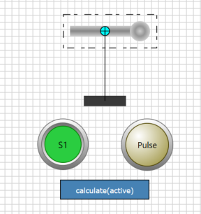
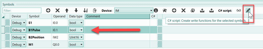
The first variant uses a calculator object with the "In Range" function. This is shown in the following example. In the example a rotary movement is realized with the help of a "revolute joint". The rotary movement depends on the operand "S1", which is influenced by a switch. The position of the rotary movement is written into the word operand "B2Position", for this this is indicated at the "Sensor Position in degrees". As soon as the rotary movement is at the position 89° to 91°, the operand "B1Pulse" should have the status 1. This is achieved via a calculator object, which is to be configured as follows:
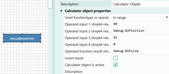
The function "In range" must be selected in the calculator object. The lower value of the range to be monitored is specified at input 1. At input 2 the operand which supplies the value and at input 3 the upper value of the range. As function result a BOOL operand is necessary, which has the status 1, as soon as the value is in the specified range. Otherwise the status 0 is written into the BOOL operand. The pulse is symbolized by a lamp. In the following the arrangement is to be seen:
Now the simulation can be started.
You can see that the lamp lights up briefly as soon as the rotary movement is within the specified range.
Generating pulses via a C# script
If you are not yet familiar with the C# script in PLC-Lab, then a description can be reached at the following link: C#-Script in PLC-Lab
In the arrangement of the above example, the calculator object is deleted and the C# script is activated.
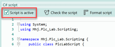
The evaluation of the range is now to be programmed in C# script. Thereby the requirement is also changed a little bit: The pulse is now to be generated 4 times per revolution. In the first step, the operands for the access are to be defined in the C# script. For this purpose, the operand "B2Position" is selected in the symbol table and the button for the read access in the C# script is pressed.
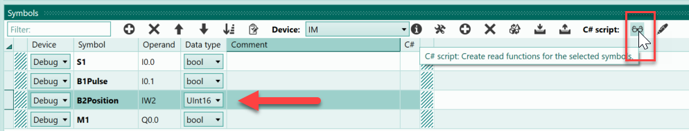
Then select the symbol or the operand "B1Pulse" and press the button for write access.
This allows the operands to be accessed in the C# script. Below is the code for the example:
public void Loop() {
    int position = (int) Get_DebugB2Position();
    //
    if (position >= 359 && position <= 360 ||
        position >= 0 && position <= 1 ||

        position >= 89 && position <= 91 ||
        position >= 189 && position <= 191 ||
        position >= 269 && position <= 271
        ){
        Set_DebugB1Pulse(true);
    }
    else {
        Set_DebugB1Pulse(false);
    }
}
At the start of the simulation, the following behavior is thus shown:
Conclusion
The two examples have shown how to use the connection for rotary movements to generate pulses. The calculator object with the "In range" function was used and the C# script. The pulses can be used, for example, for the simulation of incremental encoders.
Meaning of the property "Anchor objects collide"
As the name of the property suggests, you can make the master object and the slave object collide by activating this property. If the option is not selected, the two objects do not collide with each other. This is essential if the slave object is inside the master object.
Automatic positioning with a revolute joint (V1.5.4.0 or higher)
With the help of automatic positioning, a revolute joint can be set to a specific position. This is similar to a stepper motor control. Furthermore, positioning relative to the current position is also possible. The properties required for this functionality can be found in the "Positioning" section.
Meaning of the properties within the "Positioning" section
Enable Positioning
A Boolean operand or a constant can be specified at this property. As soon as the operand has the value '1' (true), the positioning is active. The same applies if the constant '1' is specified. If the positioning is active, the rotation can no longer be controlled via the two operands "clockwise rotation" or "counterclockwise rotation". In addition, some properties such as "Impulse behaviour" and "Reverse velocity if status of operands is zero" are deactivated. If the operand changes from '1' to '0' during positioning, the positioning is stopped.
Adopt positioning data
A Boolean operand must be specified for this property. With a pos. edge of the operand and activated positioning, the positioning process is started.
Position specification
Operand for the specification of the position increments. The value is read from the specified operand. The specification of a constant > 0 is not allowed. Depending on the positioning mode, the value is used as absolute position or relative position change. The specification of a range is not possible! A range at the position sensor of the revolution joint is used.
Position mode
Operand or constant for specifying the positioning mode to be used.
| Mode | Meaning |
|---|---|
| 0 | No function |
| 1 | Positioning via absolute value. The value at the position specification is interpreted as absolute position value. |
| 2 | Positioning via relative value. The value at the position specification is interpreted as a relative position value. The direction is determined via the property "Direction for positioning". |
Direction for positioning
Operand to specify the direction of the rotationOperand to specify the direction of the rotation while the relative positioning.
| Value | Meaning |
|---|---|
| 0 | Clockwise rotation. |
| 1 | Counterclockwise rotation. |
Sensor Positioning done
Operand becomes true as soon as a positioning job is completed. This means that the position specified by the position specification (absolute or relative) has been reached. The operand remains true until new position data is set, the position is changed or the positioning is deactivated.
Set the maximum speed for positioning
Within the section "Motor Settings" a constant or an operand can be specified at the property "Spin velocity rpm". This property is also evaluated during automatic positioning.
If the value of the operand or constant is identical to 0, then positioning is performed at maximum speed. If a value > 0 is present, then the maximum speed is limited to this value during positioning.
Example for absolute positioning
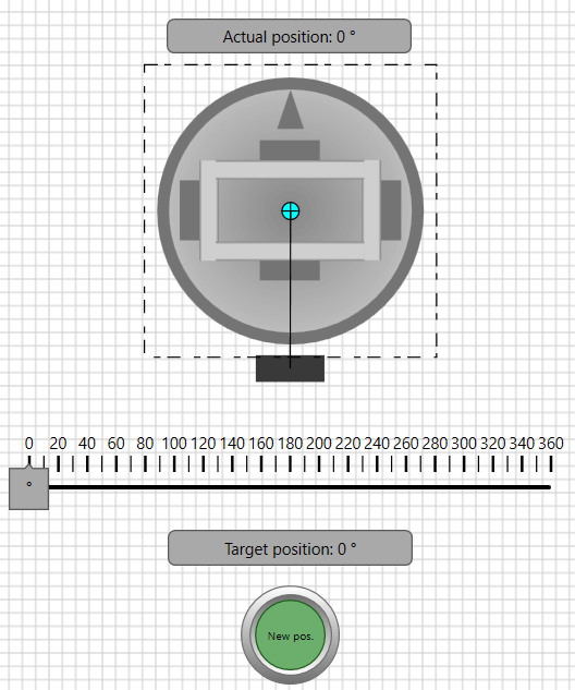
In the following example, a rotating assembly table can be positioned absolutely. Frames are machined on the assembly table and the operator can rotate the table to any position between 0 and 360°.
The assembly table is moved by means of a revolute joint. Since the position adjustment is to be made in the range 0 to 360°, no scaling is required at the "Sensor position in degrees" property. If a scaling range were necessary, the range specified at this sensor would also be used for the position data of the positioning.
The following operands are used in the example:
| Symbol | Operand | Meaning |
|---|---|---|
| GoToNewPos | E0.0 | A pos. edge of this operand starts the positioning. |
| NewPosReached | E0.1 | If the positioning is done, this operand has the status '1'. |
| ActualPos | EW2 | This word operand contains the current position of the table, in the range 0 to 360. |
| TargetPos | EW4 | The absolute target position to be approached by the table, in the range 0 to 360. |
Since the example is to run without PLC program or GRAFCET, inputs of the Sim-Device are used.
The example is installed with PLC-Lab. See also: Positioning absolute
Settings within the motor of the revolute joint
Below are the settings of the motor properties of the revolute joint.
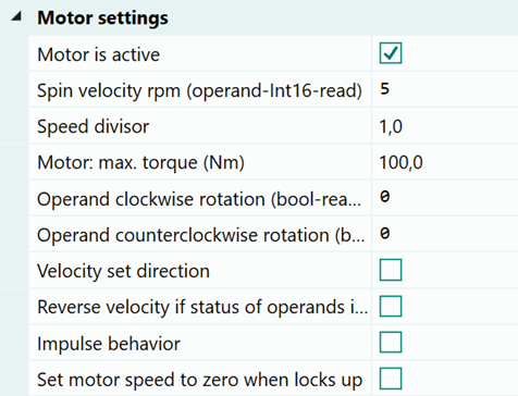
The speed is limited to 5 rpm. The properties for clockwise rotation and the counterclockwise rotation are each assigned the constant '0', as these are not used. If the table is also to be rotated manually, then the corresponding operands must be specified here. However, these would only be considered if the positioning is not active.
Settings within the sensors of the revolute joint
The only sensor required is the "Position in angle degrees" sensor. Here the operand with the symbol "ActualPos" must be specified.
Settings within the "Positioning" section
Now to the settings within the "Positioning" section. These are shown below:
The constant '1' is specified at the property "Enable positioning", because in the example the table is to be changed in position exclusively by specifying a position value. A manual change is not intended. If this were desired, then a bit operand could be specified at the property and thus switch between manual movement and automatic positioning. In the same way, the positioning could be stopped immediately with the help of the operand. This is also omitted in this example for the sake of simplicity.
The position data should be taken over at a positive edge at the operand "GoToNewPos" and the positioning should be started. Thus, this must be specified at the property "Adopt positioning data".
Since only absolute positioning is used in the example, the constant '1' can be specified in the "Positioning mode" property.
Finally, the operand "NewPosReached" must be entered at "Sensor positioning done". This operand is set to true as soon as the positioning is completed. The operand is filled in into the illuminated switch and thus signals that the position has been reached.
Simulation of the example
All settings are now complete and the system can be simulated. This can be seen below.
The position to be approached in each case is set with the aid of the slider and the positioning is started via the button. As soon as the position is reached, this is signalled by the illuminated switch.
Example for relative positioning
In the following example, a rotating assembly table is to be positioned relative to the current position. The offset to the current position can be adjusted from 1 to 100°. A rotary switch is used to select whether the movement should be to the right (clockwise) or to the left (counterclockwise).
The assembly table is moved by means of a revolute joint. Since the position adjustment is to be made in the range 0 to 360°, no scaling is required at the "Sensor position in degrees" property. If a scaling range were necessary, the range specified at this sensor would also be used for the position data of the positioning.
The following operands are used in the example:
| Symbol | Operand | Meaning |
|---|---|---|
| GoToNewPos | E0.0 | A pos. edge of this operand starts the positioning. |
| NewPosReached | E0.1 | If the positioning is done, this operand has the status '1'. |
| Direction | E0.2 | 0: Rotation clockwise, 1: Rotation counterclockwise. |
| ActualPos | EW2 | This word operand contains the current position of the table, in the range 0 to 360. |
| TargetPos | EW4 | The relative target position to be approached by the table, in the range 0 to 100. |
Since the example is to run without PLC program or GRAFCET, inputs of the Sim-Device are used.
The example is installed with PLC-Lab. See also: Positioning relative
Settings within the motor of the revolute joint
Below are the settings of the motor properties of the revolute joint.
The speed is limited to 5 rpm. The properties for clockwise rotation and the counterclockwise rotation are each assigned the constant '0', as these are not used. If the table is also to be rotated manually, then the corresponding operands must be specified here. However, these would only be considered if the positioning is not active.
Settings within the sensors of the revolute joint
The only sensor required is the "Position in angle degrees" sensor. Here the operand with the symbol "ActualPos" must be specified.
Settings within the "Positioning" section
Now to the settings within the "Positioning" section. These are shown below:
The constant '1' is specified at the property "Enable positioning", because in the example the table is to be changed in position exclusively by specifying a position value. A manual change is not intended. If this were desired, then a bit operand could be specified at the property and thus switch between manual movement and automatic positioning. In the same way, the positioning could be stopped immediately with the help of the operand. This is also omitted in this example for the sake of simplicity.
The position data should be taken over at a positive edge at the operand "GoToNewPos" and the positioning should be started. Thus, this must be specified at the property "Adopt positioning data".
Since only relative positioning is used in the example, the constant '2' can be specified in the "Positioning mode" property.
The operand "Direction" is specified at the property "Direction for positioning". If this has the status '0', the relative position change to the right (clockwise) is executed. If the operand has the status '1', then the rotation is to the left and thus counterclockwise.
Finally, the operand "NewPosReached" must be entered at "Sensor positioning done". This operand is set to true as soon as the positioning is completed. The operand is filled in into the illuminated switch and thus signals that the position has been reached.
Simulation of the example
All settings are now complete and the system can be simulated. This can be seen below.
The offset for the current position is set by means of the slider, the direction is specified and the positioning is started via the button. As soon as the position is reached, this is signalled by the button lighting up.
Examples for the revolute joint
Below you will find links to example videos in which a revolute joint was used.
Joint with a constant distance
The constant distance joint is used whenever two objects are to be connected by a rod.
This type of joint is also often used to hold parent objects at a specific location when they are multiplied by a creator. This connection can also be used to implement a pendulum.
Below you can see the principle symbol of the joint:
The following image shows two objects which are connected by a constant distance joint. The connected anchor objects are equal, i.e. there is no master or slave object for this type of connection. The connection itself is symbolized by a black line.
By simulating this structure, you can easily see the property of this joint.
Changing anchor points:
The anchor point of the joint at the respective anchor object is variable. However, it should be within the respective anchor object.
To change an anchor point, first select the line that symbolizes the joint and then click with the mouse on one of the two selection thumbs to move it. Standard anchor points appear at the respective anchor object, at which you can dock the anchor. However, anchor points at other locations within the object are also possible.
Below you can see how a new anchor point is selected:
Theoretically, you can also select an anchor point outside of an anchor object. But then the behavior of the joint is no longer completely clear and the physical simulation may be unstable.
"Rigidity" and "Damping" Properties:
At the beginning we mentioned that a constant distance joint is comparable to a rod connecting two objects. With the two properties "Rigidity" and "Damping" the nature of the joint can be changed slightly.
The "Rigidity" property can take values from 1 to 30. 1 is soft and 30 is rigid. The default value is 29.
If the value 1 is selected here, the connecting rod is converted into a connecting chain, but with relatively large chain links.
The property "Damping" can take the values 0.0 to 1.0. The default value is 0.9. This allows the nature of the joint to be varied between metal and hard rubber.
Examples for constant distance joints:
Below you will find links to example videos in which a constance distance joint was used.
Solid joint
A solid joint is used when two objects are to be connected inseparably.
This type of joint is also used when one or more objects are to be attached to the piston rod of a cylinder.
There may also be gaps between the two objects connected by the joint. The gaps are permeable for other objects, similar to a sieve.
Below you can see the principle symbol of the joint:

In the following image, two objects are connected by solid joint. The left object is the master object. Drawing of the joint was started with this object. The slave object (circle) is located on the right.
You can see that the connection symbol on the side to the master object is represented by a solid line, while the line to the slave object is represented by a dotted line.
When the joint is created, some properties of the master object are adopted by the slave object. For this reason, you should assign the role of the master object to the "more dominant" object and start drawing the joint with it.
If, for example, another object is attached to the piston rod of a cylinder, then the piston rod should be the master object.
But in many cases the role distribution has no influence on the function of the joint.
The difference between a body group and a solid joint:
In the PLC-Lab action window you will find the section "Body group". There you will find the action "Create a body". This action creates a body from the currently selected objects. This is symbolized by a body group, which is surrounded by a dashed rectangle. The border is different from a drawing group.
So the action "Create a body" has the same effect as joining to a body. This raises the question of when to use the joint and when to use the action.
To simplify, you can say that if more than two objects are to be combined to a body, the action "Create a body" should be used. If, for example, such a body group is to be firmly connected with another object, then the solid joint should be used
The following video shows this very clearly. A container is built with the help of a body group and then attached to the piston rod of the cylinder with a solid joint.
In principle, you could also implement the container with the help of several solid joints. This would also work.
The other advantage of the body group, in particular where numerous objects are involved, is that it behaves like a drawing group. This means that you can, for example, zoom in and out while maintaining the relative position of the objects to each other. If an object within the group is copied with the mouse, then the newly created object is also part of the group and thus part of the body.
The disadvantage of the body group is if objects that do not belong to the body are arranged within the group. In this case it is not obvious that these objects do not actually belong to the body. Here a solid joint would be better because the symbols of the joint visually indicate the affiliation.
Body groups are explained in more detail at the following link:
Gaps between objects that form a body:
We have already mentioned that there can be gaps between objects that are combined to form a body.
This further increases the flexibility in the construction of virtual facilities.
Example
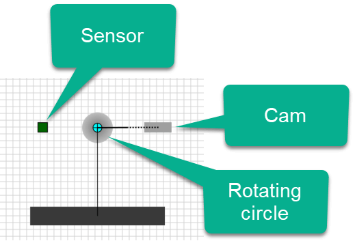
The following example shows a layout in which a cam is attached to a rotating circle object which actuates a sensor. The sensor was not placed directly on the circle object.
The simulation of the layout shows the following behavior:
You can see that the cam rotates with the circle object. The gap between the circle object and the cam has no influence on the joint.
Example
In the second example, a rocker was built from individual rectangles. The rectangles were combined into one body with the help of a body group. The bottom of the rocker resembles a sieve, which means it has gaps. On the rocker you will find a circle objects, which by their size fall through the gaps of the sieve. The rocker can be moved using buttons.
You can see that the circle objects fall through the gaps. Despite the gaps, the rectangles form a body.
Conclusion
Objects that are combined to one body can also be spatially separate from each other. Despite this separation, they react as if a joint exists. This "virtual" joint does not influence other objects.
Weld joint (removable)
A weld joint is used when two objects are to be connected to each other. In contrast to the "solid joint", however, this joint can be removed again.
For this purpose, a force or strength can be specified for a weld joint. If a greater force acts on the joint, then the joint "breaks" and no longer exists.
Below you can see the principle symbol of the joint:

In the following image, two objects are connected by a weld joint. In the case of a weld joint, there is no master or slave object. The joint is symbolized by a solid line with a circle in the center.
The ends of the weld joint are the fixing points on the respective anchor object. When the simulation is started, the force of the weld joint acts at these fixing points. For the above image, this means that the two objects are joined at these points. The following image shows this.
Changing the fixing points on the anchor objects:
If you want to change the fixing points of the anchor objects, proceed as follows:
- Select the weld joint.
- Move the thumb of the anchor object that you want to change with the mouse.
You can see this below.
As soon as you "touch" the thumb with the mouse, the standard points of the respective anchor object become visible for docking. However, you don't have to use these. You can choose the placing freely.
If you switch on the simulation after the above selection of the fixation point, the following behavior is indicated:
The corner point at the bottom right is now the point at which the force of the weld joint acts.
Example
In the example, the weld joint is placed as follows:
The setting was made so that the two anchor objects don't collide.
When the simulation is switched on, the following behavior is indicated:
The force of the weld joint acts at the respective center of the anchor objects and pushes them together. Again, this behavior is only possible if the anchor objects do not collide.
Example In the next example, the fixing points are located outside the anchor objects.
This creates a gap between the two at the start of the simulation.
However, the anchor objects are still connected to each other via the weld joint.
Setting the maximum force of the weld joint:
A weld joint can be "destroyed" or "broken" if it is subjected to a force that is greater than the maximum force set for the joint.
The following properties must be set in order to make the weld connection removable:
- Select the property "Joint is breakable" in the section "Physics properties -> General".
- Adjust the maximum force in the property "Max. force before the joint is breaking" in the section "Physics physics properties -> General".
Example
In the example shown below, we have set the weld joint to break at a maximum force of 10N.
The connected anchor objects fall from above onto a pointed object. The resulting force causes the weld joint to break. As a result, the two anchor objects are separated from each other.
Welding and releasing objects by touching them:
Above we have shown that a weld joint can be set to break. The force acting on the joint must be greater than or equal to the set maximum force.
For geometric objects (rectangle, ellipse, triangle), the "Weld joint" section is available. There are two properties in this section.
The property "Operand create weld joint":
This property expects a bit operand or an operand with a range specification (../see also Specification of a range in addition to the operand). Because the value is read from the operand, the constant '1' can also be specified. In this way, the function of the property is always active.
If the property of a physics object is active and this object collides with two other physics objects, then these are welded at the point of collision.
Example
In the following example, two dynamic rectangles are to be welded using a cylinder. For this purpose, a dynamic rectangle is attached to the cylinder rod of the cylinder (with an unbreakable joint) in which the property "Operand create weld joint" has been assigned the constant '1'. As a result, the property is permanently active.
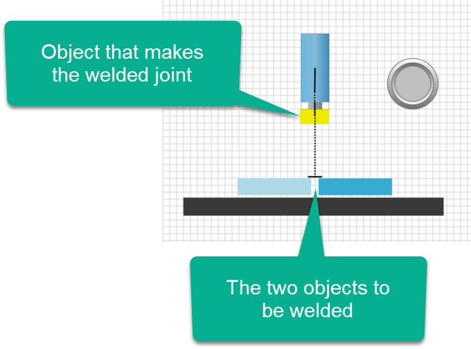
The cylinder can be moved downwards by means of a push-button. In the lower end position of the cylinder, the welding object touches the two rectangles to be welded.
Below you can see the effect.
Initially, the two rectangles are still independent of each other. The two rectangles are only connected after the cylinder has reached its lower end position and the object on the cylinder rod has carried out the welding process.
The property "Operand remove weld joint":
This property expects a bit operand or an operand with a range specification (../see also Specification of a range in addition to the operand). Because the value is read from the operand, the constant '1' can also be specified. In this way, the function of the property is always active.
If the property of a physics object is active and this object collides with two other physics objects, which were joined together by means of the property "Operand remove weld joint", then they are separated again.
Example
In the following example, a similar arrangement is used as with the example for the property "Operand create weld joint". In this example, the object on the piston rod of the cylinder is adjusted so that the welding and removing of a joint can be switched over.
You can see how the two rectangles are first welded together. Then the function of the object on the piston rod is switched from "weld" to "remove". After the cylinder has moved downwards, the two rectangles have been separated again. The weld joint has thus been eliminated.
Info
Note: It is not possible to remove weld joints which have been defined graphically using a weld joint. Only the joints created using the property "Operand create weld joint" can be removed using "Operand remove weld joint".
Videos on both properties:
Below is a link to a video illustrating the use of the two properties to create and remove a weld joint.
Wheel joint with shock absorber
As the name suggests, this joint is mainly used when a wheel joint with a shock absorber is required.
The pivot point of the joint can be changed within the limits of the joint symbol.
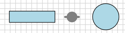
Below you can see the principle symbol of the joint:
When you create the joint, you have to start with the object that represents the fixed part of the wheel joint. The second anchor object is the rotating slave object.
The following image shows two objects which are connected by a "wheel joint". The lower object is the master object, which in many cases will be a fixed object. From the master object, a slightly wider solid line leads to the center of the joint symbol. Also from the center of the joint symbol, a slightly thinner line leads to the slave object.
The circle indicates the pivot point. The slave object is the object that rotates around this pivot point.
Changing the position of the pivot point in the "wheel joint":
You can change the pivot point of the joint. To do this, select the symbol of the joint and move the circle or its thumb with the mouse. In the following example, the pivot point is placed in the center of the slave object.
Now an example where the pivot point is placed outside the slave object.
The examples show that very different rotary movements can be implemented by shifting the pivot point.
Using the "wheel joint" motor:
The joint has a motor that can be set using the "Motor" property in the property section "Physics properties -> General -> Motor settings". The motor speed (in rpm) can be specified via an operand; the value is read from the operand. In this way, it is also possible to specify a constant if the speed does not have to be variable.
With the property "Speed divisor" you can adapt the speed specification for the simulation by means of an operand without having to change the value of the operand. The speed specified in the operand is divided by the value in "Speed divisor". This may be necessary, for example, if the motion is too fast in reality and therefore cannot be recreated in the simulation.
The right/left rotation of the slave object is controlled via operands. Because the value is read from the operand, the constant '1' can also be specified for a permanent rotation. Please note, however, that only one direction of rotation may be active at any one time. If both directions of rotation are active, there is no rotary movement.
Limit switches and sensors for a "wheel joint":
The joint has numerous sensors. A separate sensor detects the amplitude of the joint's shock absorber. The standard values are -100% (completely extended) to 100% (completely compressed). By specifying a range, it is possible to scale these values to other values. This sensor is often used to detect the unbalance of a rotation.
The "rigidity" and "damping" can be varied by the properties of the same name.
The following video shows an example for this type of use:
Meaning of the property "Anchor objects collide":
As the name of the property suggests, you can make the master object and the slave object collide by activating this property. If the option is not selected, the two objects do not collide with each other. This is essential if the slave object is inside the master object.
Changing anchor points:
The anchor point of the joint at the respective anchor object is variable. However, it should be within the respective anchor object. To change an anchor point, first select the symbol the joint and then click with the mouse on one of the two selection thumbs to move it. Standard anchor points appear at the respective anchor object, at which you can dock the anchor. However, anchor points at other locations within the object are also possible.
Below you can see how a new anchor point is selected: